Import standard modules:
import numpy as np
import matplotlib.pyplot as plt
%matplotlib inline
from IPython.display import HTML
HTML('../style/course.css') #apply general CSS
Import section specific modules:
import matplotlib.image as mpimg
from IPython.display import Image
HTML('../style/code_toggle.html')
1.11 Modern Interferometric Arrays
In the previous sections of this chapter we have covered the motivation for using interferometry to make measurements, the observable astrophysics and cosmology in the radio regime, and why interferometry is used in radio astronomy. This final section provides an overview of some of the interferometric arrays currently in use, the science goals of these projects, and future arrays in development.
As the scale and cost of science in physics has grown there is a drive for international collaboration to pool resources in order to build large, multi-purpose arrays. These arrays are meant to run as long term observatories with astronomers requesting time for a proposed projects. The prime example of this type of array is the future Square Kilometre Array (SKA). Another array type is an ad-hoc array such as in very-long baseline interferometry (VLBI) where single dish telescopes (or beamformed arrays) from all over the world are combined (via a signal recorder) for an observation. The recorded signals are later sent to a correlator to create an interferometric observation. There are also experiment-driven arrays which are focused on a single experimental outcome with a limited lifetime. Many of the Epoch of Reionization (EoR) arrays follow this model.
1.11.1 Karoo Array Telescope (MeerKAT/KAT-7)
MeerKAT, and it's precursor KAT-7, is an South African developed observatory located in the Northern Cape of South Africa. MeerKAT will be a one of the premier telescope arrays and be central to the development of the Square Kilometre Array (SKA).
The Karoo Array Telescope, or KAT-7, is a 7 dish intereferometric array. It was designed as a prototype system for the MeerKAT array (currently in construction and commissioning). KAT-7 was constructed from 2009 to 2011, and will remain running for the near future. Designed primarily as an engineering prototype it has also been used for science observations. Much of this book uses KAT-7 examples as it is simple enough to understand yet was designed with modern technology. The current status and specifications for the array can be found here⤴.
Image(filename='figures/arrays/kat7_dish_2013.jpg')

Figure 1.11.1: KAT-7 prime-focus telescope. Credit: SKA South Africa⤴
Each of the elements is a 12 meter, prime-focus (the receiver is at the focal point of the dish) parabolic dish. If a single element would be used for an oberservation it would have a resolution of about a degree for the freqeuncy band the receivers operate at. The important dish specifications are in the table below.
| Dish Specifications | |
|---|---|
| Optics | Prime Focus |
| Diameter | 12 m |
| $\Delta \theta_{1.4 GHz}$ | 1.22 deg |
The resolution of the dish $\Delta \theta_{1.4 GHz}$ (also called the primary beam) is presented at 1.4 GHz, that is the 21 cm Hydrogen hyperfine transition line. This is a common observing frequency, so it will be used as a comparision between many of the arrays in this section.
The KAT-7 receiver band covers the observing range 1.2 GHz to 1.95 GHz, the digital hardware is capable of processing 256 MHz of this band instantenously, i.e. at any given time. This frequency range is called L-banb in reference to the radio communication spectrum allocation labels. The L-band receiver feed is a dual-polarization, linear system, polarization will be covered in Chapter 7. The receiver specifications are in the table below.
| Recievers | |
|---|---|
| Band | L |
| $T_{sys}$ | $< 35 K$ |
| Start Frequency | 1200 MHz |
| Stop Frequency | 1950 MHz |
| Total Bandwidth | 750 MHz |
| Instantaneous Bandwidth | 256 MHz |
| Fractional Bandwidth | 0.14 - 0.19 |
| Polarization | Dual Linear |
A common method to describe the bandwidth of a receiver system is to use the fractional bandwidth $\nu_{\textrm{frac}}$ is
$$\nu_{\textrm{frac}} = \frac{\nu_f - \nu_0}{\nu_c}, \quad \nu_c = \frac{\nu_f + \nu_0}{2},$$where $\nu_f$ is the highest frequency of the band and $\nu_0$ the lowest frequency. The center frequency $\nu_c$ is the average of $\nu_f$ and $\nu_0$. The fractional bandwidth is often used to compare receivers at different frequencies as $\nu_{\textrm{frac}}$ is independent of frequency.
The instantaneous bandwdith is split into frequency channels (or sub-bands) in digital hardware. The specifics of this channelization and band selection depend on the science observation. But for a typical 'wideband' observation the frequency channels have a bandwidth of 390 kHz.
The system temperature $T_sys$ is an average measure of the sensitivity of the telescope, the lower the temperature the better, this is discussed in Chapter 7.
The array layout is what would be called 'compact' in that the telescopes are close to each other, thus the synthesized KAT-7 telescope has limited resolution. As there are only 7 elements in the array the visibilty sampling (uv coverage) is sparse. The telescopes are randomly distributed to partially compensate for the sparseness. The topics of uv coverage and distribution will be covered in later chapters.
Image(filename='figures/arrays/kat7_2016_aerial.jpg')

Figure 1.10.2: KAT-7 array layout, located in the Northern Cape of South Africa. Credit: SKA South Africa⤴
If we think of the array as a synthesized telescope then we can think of that telescope having a maximum resolution based on the maximum baseline length, in the case of KAT-7 that is 185 meters, which at 1.4 GHz translates (via the Rayleigh criterion) to a resolution of 4.7 arc-minutes. Interetestingly, we can also think of the array as having a minimum resolution based on the minimum baseline length. Two elements can never be closer then their size, otherwise they would need to physically overlap. The effect of a minimum baseline, as we will see in later chapters, is that interferometric arrays are not sensitive to 'large-scale' structure, e.g. the galactic synchrotron structures. A single element telescope, which is not limited by this minimum resolution effect, can be used to complement interferometric observations ⤴.
| Array Specifications | |
|---|---|
| Number of Elements | 7 |
| Min Baseline | 26 m |
| Min $\Delta \theta_{1.4 GHz}$ | 0.56 deg |
| Max Baseline | 185 m |
| Max $\Delta \theta_{1.4 GHz}$ | 4.7' (0.08 deg) |
The main goals of KAT-7 were engineering-driven, but a number of science results continue to be produced by observation using the array. As MeerKAT is built out and commissioned KAT-7 projects will come to a close. As of this writing the MeerKAT array is under construction, check here⤴ for the current status and main scientific project plan.
Image(filename='figures/arrays/meerkat_dish_2015.jpg')

Figure 1.10.3: MeerKAT offset-Gregorian telescope, without the feed system instelled. Credit: SKA South Africa⤴
The 13.5 meter MeerKAT dish is markedly different from the prime-focus KAT-7 design. The MeerKAT dish has offset Gregorian optics, the results in a 'better' beam pattern. Different optics and beam patterns is discussed in Chapter 7. This optics design will be the basis for the mid-frequency SKA dishes.
| Dish Specifications | |
|---|---|
| Optics | Offset Gregorian |
| Diameter | 13.5 m |
| $\Delta \theta_{1.4 GHz}$ | 1.09 deg |
There are currently two tested receiver bands for MeerKAT, and L-Band receiver similar to KAT-7 and a lower frequency Ultra High Frequency (UHF) receiver. Both recevier bandwidths are fully sampled by the digital hardware leading to an instantaneous bandwidth which is larger than the total bandwidth. We only consider the total bandwidth as the digital bandwidth will sample a region of the frequency band with no signal as those regions have been filtered out.
| Receivers | ||
|---|---|---|
| Band | UHF | L |
| $T_{sys}$ | $< 38 K$ | $< 30 K$ |
| Start Frequency | 580 MHz | 900 MHz |
| Stop Frequency | 1015 MHz | 1670 MHz |
| Total Bandwidth | 435 MHz | 770 MHz |
| Instantaneous Bandwidth | 544 MHz | 856 MHz |
| Fractional Bandwidth | 0.55 | 0.6 |
| Polarization | Dual Linear | Dual Linear |
The MeerKAT array layout follows a random distribution with a dense core. The randomness imrpoves the $uv$ coverage while the dense core is desirable for many of the science goals. The array core, shown below, is currently being populated with dishes and receiver systems.
Image(filename='figures/arrays/meerkat_2016_aerial.jpg')

Figure 1.10.4: MeerKAT array core layout, located in the Northern Cape of South Africa, currently under construction. Credit: SKA South Africa⤴
The array is made up of 64 dishes, with a shortest baseline similar to KAT-7, but with a maximum baseline of 8 km! This will allow for high resolution, up to 6.6 arc-second, measurements.
| Array Specifications | |
|---|---|
| Number of Elements | 64 |
| Min Baseline | 29 m |
| Min $\Delta \theta_{1.4 GHz}$ | 0.51 deg |
| Max Baseline | 8 km |
| Max $\Delta \theta_{1.4 GHz}$ | 6.6" |
MeerKAT will be a general purpose interferometric observatory, as such there are a number of different planned science surveys⤴.
1.11.2 Jansky Very Large Array (JVLA)
The Karl G. Jansky Very Large Array (JVLA)⤴ is the latest upgrade (2011) to the original Very Large Array (1975). The 27 element array is located in New Mexico, USA and operated by the NRAO. The JVLA is the quintessential radio interferometric array and is the standard in which other array are measured. It is typical to see an interferometric array sensitivity or resolution presented are a fraction of the JVLA. Details on the array specifications, such as resolution, sensitivity, correlation configuration, etc. can be found here⤴.
Image(filename='figures/arrays/vla_dish_2007.jpg')

Figure 1.11.5: JVLA cassegrain-focus telescope. In the foreground are tracks used to move telescopes to different positions. Credit: Wikimedia Commons⤴
The 25 meter JVLA dishes use a Cassegrain optical system for most of the receivers (though a low-frequency receiver is at the focal point). Cassegrain optics uses a secondary reflector, at the focal point to redirect the signal to the recievers at the base of the dish.
| Dish Specifications | |
|---|---|
| Optics | Cassegrain |
| Diameter | 25 m |
| $\Delta \theta_{1.4 GHz}$ | 0.59 deg |
There are numerous receiver systems⤴, all circular polarization, on each telescope which are cycled through depending on the observation and configuration schedule. The receivers cover most of the frequency range⤴ between 58 MHz and 50 GHz. Correlation of visibilities is done with the flexible WIDAR⤴ correlator. As there are many frequency bands and different correlion options the bandwidth parameters are not included in the table below.
| Receivers | ||||||||||
|---|---|---|---|---|---|---|---|---|---|---|
| Band | 4 | P | L | S | C | X | Ku | K | Ka | Q |
| SEFD | 10000+ Jy | 2790 Jy | 420 Jy | 370 Jy | 310 Jy | 250 Jy | 350 Jy | 560 Jy | 710 Jy | 1260 Jy |
| Start Frequency | 58 MHz | 230 MHz | 1 GHz | 2 GHz | 4 GHz | 8 GHz | 12 GHz | 18 GHz | 26.5 GHz | 40 GHz |
| Stop Frequency | 84 MHz | 470 MHz | 2 GHz | 4 GHz | 8 GHz | 12 GHz | 18 GHz | 26.5 GHz | 40 GHz | 50 GHz |
| Total Bandwidth | 26 MHz | 240 MHz | 1 GHz | 2 GHz | 4 GHz | 4 GHz | 6 GHz | 8.5 GHz | 13.5 GHz | 10 GHz |
| Polarization | Dual Circular | Dual Circular | Dual Circular | Dual Circular | Dual Circular | Dual Circular | Dual Circular | Dual Circular | Dual Circular | Dual Circular |
The sensitivity⤴ of receivers is presented in System Equivalent Flux Density (SEFD) which is a function of the system temperature $T_{sys}$ and the efficiency of the telescope $\eta$. Part of the efficiency measurment is the reflectivity of the dish, at higher frequencies the reflectivity drops off and the dish becomes more inefficient. This accounts for the increase in SEFD at the higher frequency receivers. The extreme increase in SEFD at the lower end is because the sky temperature (mainly due to synchrotron) increases at low frequencies. Sensitivity is discussed in Chapter 7.
Image(filename='figures/arrays/vla_aerial.jpg')

Figure 1.11.6: JVLA array layout in the densest (D) configuration. Credit: NRAO/AUI⤴
The JVLA elements are laid out on a 'Y'-shape, each arm of the 'Y' is made of two sets of rail tracks which allows the elements to be repositioned into different configurations⤴ to result in different resolution⤴ measurements. The four configurations (A, B, C, D) are set configurations which vary the maximum and minimum baseline length (shown in the table below). The A configuration has the highest resolution, but is limited in low resolution, while D configuration is the densest layout and is most sensitivty to low resolutions. The same field in the sky can be observed with different configurations, the measured visibilties can be combined to form an image sensitive to all resolutions scales from A to D configuration. These configurations are cycled through on a standard schedule.
| Array Specifications | A | B | C | D |
|---|---|---|---|---|
| Number of Elements | 27 | 27 | 27 | 27 |
| Min Baseline | 680 m | 210 m | 35 m | 35 m |
| Min $\Delta \theta_{1.4 GHz}$ | 1.3' | 4.2' | 25.2' | 25.2' |
| Max Baseline | 36.4 km | 11.1 km | 3.4 km | 1.03 km |
| Max $\Delta \theta_{1.4 GHz}$ | 1.5" | 4.8" | 15.5" | 51.3" |
As the JVLA, in some form, has been around for decades an enormous amount of scientific research has been produced. We will not even attempt an overview of the work that has been produced. But, as an entry point, one of the defining surveys using the VLA is the NRAO VLA Sky Survey (NVSS) ⤴ which is a classic radio catalogue.
1.11.3 Australian Square Kilometre Array Pathfinder (ASKAP)
On the path to developing the SKA, along with MeerKAT, the Australian Square Kilometre Array Pathfinder (ASKAP) is under construction in western Australia. This array uses a phased-array feed (PAF) receiver which effectively expands the field of view, allowing for a number of scientific advantages. As PAFs are a new technology ASKAP will act as an engineering testing ground while also doing scientific observations. The update to date system specifications can be found here⤴.
Image(filename='figures/arrays/askap_dish_2015.jpg')

Figure 1.11.7: ASKAP phased-array feed telescope. Credit: CSIRO⤴
At the prime focus of each dish is a PAF which is used to form multiple 'beams' and increase the effective field of view of the dish. The dish mount has a 'third-axis' which corrects for the rotation of the PAF due to change in parallactic angle. This axis is necessary to keep the PAF 'beams' fixed to a position in the sky. The details of PAFs are not covered in this book, for those interested see the Phased Array Antenna Handbook ⤴.
| Dish Specifications | |
|---|---|
| Optics | Prime Focus |
| Diameter | 12 m |
| $\Delta \theta_{1.4 GHz}$ | 1.22 deg |
The PAFs operate at L-band, they have a higher system temperature and smaller bandwidth coverage compared to MeerKAT, but can make up for this in survey science by covering a larger field of view for a fixed time.
| Receivers | |
|---|---|
| Band | L |
| $T_{sys}$ | $50 K$ |
| Start Frequency | 700 MHz |
| Stop Frequency | 1800 MHz |
| Total Bandwidth | 1100 MHz |
| Instantaneous Bandwidth | 300 MHz |
| Fractional Bandwidth | 0.18 - 0.35 |
| Polarization | Dual Linear |
The phased-array feeds have been upgraded to a second generation version, which has greatly reduced the system temperature compared to the first generation. Below is a close-up of the first generation 'checker board' PAF. The green panel is an active component which is used to form multiple digital beams.
Image(filename='figures/arrays/askap_paf_2010.jpg')

Figure 1.11.8: Close up of the mark-I phased-array feed on ASKAP. Credit: CSIRO/David McClenaghan⤴
ASKAP is made up of 36 elements, with a similar minimum and maximum baseline distribution to MeerKAT. The layout of the array can be found here⤴.
| Array Specifications | |
|---|---|
| Number of Elements | 36 |
| Min Baseline | 37 m |
| Min $\Delta \theta_{1.4 GHz}$ | 0.39 deg |
| Max Baseline | 6 km |
| Max $\Delta \theta_{1.4 GHz}$ | 8.8" |
Again, similar to MeerKAT there are a number of survey science projects⤴ planned for when the array has been commissioned.
1.11.4 The Low-Frequency Array (LOFAR)
Stepping away from traditional dish-based interferometry we will take a look at the Low-Frequency Array (LOFAR)⤴ which was designed and build by the Dutch national astronomy research foundation ASTRON. This is a unique array as it is made up of stations instead of dish telescopes. Each station is made up of simple antenna elements and beamformed to act as a single telescope. These stations are called aperture arrays. They have the advantage of being 'electronically-steerable' which means that without any physical moving parts the aperture array can be 'pointed' in any direction in the sky. This is possible using the station digital electronics. This technique allows the aperture array to be pointed in multiple locations at the same time, something not possible with a dish optics system. LOFAR operates at a low frequency (< 250 MHz) compared to the arrays we have discussed so far. As such it has opened up a new region of the observable parameter space.
Image(filename='figures/arrays/lofar_uk_station.jpg')

Figure 1.11.9: Aperture array LOFAR-UK⤴ international station at Chilbolton Observatory. The High-Band Array (black flat structure in the top-left) made up of 96 titles, each tile is composed of 16 'bowtie' dual-polarization dipole elements. The Low-Band Array (square patches in the foreground) is made up of 96 dual-polarization 'droopy' dipole elements (see figure below). The digital electornics to 'point' the stations is located in the small grey bunker. Credit: LOFAR-UK/D. McKay-Bukowski⤴
Each station contains two arrays. The High-Band Array (HBA) operates from 100 MHz to 250 MHz, and is made up of 'tile' elements. These tile elements are themselves made up of 16 'bowtie' dipole antenna elements. The signals from each bowtie is combined via an electronic beamformer, the titles are then further beamformed into a single signal. This signal is sent to a central correlation and computing cluster in the Neatherlands. The Low-Band Array (LBA) operates from 0 to 100 MHz and is made up of 'droopy' dipole elements (shown below). Similar to the HBA the signal from all the elements is beamformed and sent to the main computing centre. The station can also act as indepenedent array and interferometry can be done using only the station elements.
Image(filename='figures/arrays/lofar_lba_element.jpg')

Figure 1.11.10: Low-Band Array (LBA) 'droopy' dipole antenna elements. These elements are combined as an aperture array to function as an electronically-steerable telescope. Credit: ASTRON⤴
LOFAR operates in different observing modes⤴ depending on the project. The station configuration varies depending on if the station is located in the core, the Netherlands, or at international locations, details on the station layout can be found here⤴.
At low frequencies the system temperature is dominated by the sky temperature, this allows for cheap, room temperature components to be used as this will result in a relatively small increase in the system noise. The response of the antenna elements varies over the large fractional observing bandwidth which resulting in a sensitivity⤴ which depends on observing frequency and pointing.
| Recievers | |||
|---|---|---|---|
| Band | LBA | HBA-Low | HBA-High |
| Start Frequency | 0 MHz | 100 MHz | 200 MHz |
| Stop Frequency | 100 MHz | 200 MHz | 250 MHz |
| Total Bandwidth | 100 MHz | 100 MHz | 50 MHz |
| Instantaneous Bandwidth | 96 MHz | 96 MHz | 96 MHz |
| Fractional Bandwidth | 2 | 0.67 | 0.22 |
| Polarization | Dual Linear | Dual Linear | Dual Linear |
As of February 2016 there was 45 stations in operation, but the modular station design allows for more stations to be build. The majority of the stations are located in the Netherlands (see figure below). The international stations allow for high resolution interferometric observations.
Image(filename='figures/arrays/lofar_station_map_oct_2015.png')

Figure 1.11.11: LOFAR station locations and status as of October 2015. The core and superterp are located near Exloo, Netherlands. Credit: ASTRON/George Heald⤴
LOFAR is a unique array as it operates in a frequency band which has been under-observed in the past. It complements higher frequency arrays (like the JVLA). It is currently in an observing schedule focused on the selected key science projects⤴.
1.11.5 Atacama Large Millimeter/submillimeter Array (ALMA)
Going in the other frequency direction to LOFAR is Atacama Large Millimeter/submillimeter Array (ALMA)⤴ which is a high frequency array located in the Atacama Desert in Chile at around 5000 meters. This elevation is useful for high frequency (> 50 GHz) radio astornomy as the water vapor in the atmosphere and tropospheric effects have detrimental effects on observations. ALMA is a collaboration between the NRAO in the US, NAOJ in Japan, and ESO in Europe.
Image(filename='figures/arrays/alma_dishes.jpg')

Figure 1.11.12: The four types of ALMA antennas: European, North American and Japanese 12 meter telescope, along with a 7 meter diameter one. Credit: ALMA (ESO/NAOJ/NRAO), W. Garnier (ALMA)⤴
ALMA consists of two dish sizes (12 m and 7 m), the smaller dishes make up the compact core at the centre of the array. As the array operates at very high frequency the dish surfaces must be very accurate to have a significant reflector efficiency. Many of the telescopes can also be moved around, this requires accurate knowledge of the telescope positioning.
| Dish Specifications | ||
|---|---|---|
| Optics | Prime Focus | Prime Focus |
| Diameter | 12 m | 7 m |
| $\Delta \theta_{\textrm{Band 9}}$ | 9.3" | 16" |
Like the JVLA, ALMA operates across a wide range of frequencies (broken into bands), but at a higher frequency. The lowest frequency bands 1-3 are planned but not yet built. The ALMA bands start around the highest frequencies of the JVLA and go up to near the limit of heterodyne detectors in the far-infrared. Though the bands cover significant frequency ranges compared to the lower frequency arrays many of the bands have similar fractional bandwidth. The instantaneous bandwidth is limited by the correlator system to 8 GHz (it is an impressive correlator).
| Recievers | ||||||||||
|---|---|---|---|---|---|---|---|---|---|---|
| Band | 1* | 2* | 3* | 4 | 5 | 6 | 7 | 8 | 9 | 10 |
| $T_{sys}$ | 17 | 30 | 37 | 51 | 65 | 83 | 147 | 196 | 175 | 230 |
| Start Frequency | 31 GHz | 67 GHz | 84 GHz | 125 GHz | 162 GHz | 211 GHz | 275 GHz | 385 GHz | 602 GHz | 787 GHz |
| Stop Frequency | 35 GHz | 90 GHz | 116 GHz | 163 GHz | 211 GHz | 275 GHz | 373 GHz | 500 GHz | 720 GHz | 950 GHz |
| Total Bandwidth | 4 GHz | 23 GHz | 32 GHz | 38 GHz | 49 GHz | 64 GHz | 98 GHz | 115 GHz | 118 GHz | 163 GHz |
| Instantaneous Bandwidth | 8 GHz | 8 GHz | 8 GHz | 8 GHz | 8 GHz | 8 GHz | 8 GHz | 8 GHz | 8 GHz | 8 GHz |
| Fractional Bandwidth | 0.12 | 0.29 | 0.32 | 0.26 | 0.24 | 0.26 | 0.30 | 0.26 | 0.18 | 0.19 |
ALMA consists of 66 dishes, with short wavelength observing frequnecies and long baselines the array can resolve milli-arcsecond structure.
| Array Specifications | |
|---|---|
| Number of Elements | 66 |
| Min Baseline | ~150 m (compact config) |
| Min $\Delta \theta_{\textrm{Band 9}}$ | 0.7" |
| Max Baseline | ~16 km (extended config) |
| Max $\Delta \theta_{\textrm{Band 9}}$ | 6 mas |
Image(filename='figures/arrays/alma_core_layout.jpg')

Figure 1.11.13: ALMA core layout on the Chajnantor Plateau in Chile, made up of 12 m and 7 m telescopes, some of the telescopes can be repositioned to change the visibility sampling, similar to the VLA. Credit: ALMA (ESO/NAOJ/NRAO), O. Dessibourg⤴
Much of this book focuses on lower frequency interferometry, but the same principles apply to doing interferometry with an array like ALMA. The fundamentals remain true for all interferometric arrays, though the details change.
1.11.6 VLBI Networks
Moving beyond the purpose built arrays we have covered so far there are also interferometry networks. The idea behond a network is that multiple telescopes which normally operate in a single-dish observation mode can observe the same position in the sky and record the signals at the same time. These signals are then sent to a central location where they are correlated to produce visibilities. This ad-hoc network design is most widely used in very long baseline interferometry (VLBI) which uses telescopes from all over the world to create a synthesized telescope on the scales of the Earth. VLBI can be used to perform the highest resolution astronomy such as measuring the size-scale of super-massive black holes at the centre of galaxies (Event Horizon Telescope⤴, BlackHoleCam⤴).
VLBI is incredibly difficult to do, as it requires very accurate knowledge about time and positions of the telescopes. These telescopes are on different in different parts of the world, and though we may think of land and continents as being static, they are, of course, moving at rates of millimeters per year. These movements are taken into account with VLBI observations along with many other details. It is truly an engineering and scientific feat.
There are multiple VLBI networks, and they vary in size scale from the scale of a country (eMERLIN⤴) to supa-continental (EVN⤴, VLBA⤴). For example, the European VLBI Network (EVN) includes most major radio telescopes in Europe but also includes ttelescopes in Africa, Asia, and North America (see figure below).
Image(filename='figures/arrays/evn_map.png')

Figure 1.11.14: Locations of telescopes in the European VLBI Network. Credit: EVN⤴
Now, give the physical limations of the Earth one might think that there is a hard limit on the maximum distance between two telescopes. But, it is possible to do longer baseline interferometry by putting telescopes in orbit to do Space VLBI. RadioAstron⤴ is an ongoing project to use a space-based radio telescope to do interferometry with ground-based telescopes. Space-based interferometry will happen at some point in the future. In the context of very low-frequency (< 10 MHz) radio astronomy it will be a necessity due to ionospheric reflection.
1.11.7 Epoch of Reionization Arrays
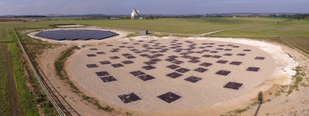
The interferometric arrays discussed so far has been multi-purpose arrays, though they may have specific key science goals, these arrays can be used for many different types of observations. There are also purpose built arrays which are primarily designed for a specific experiment. Such is the case with Epoch of Reionization (EoR) arrays. These are low-frequency (observing at > 200 MHz) arrays which are being used to detect the redshifted Hydrogren 21 cm line which is a tracer for the evolution of the universe during the epoch of reionization. These arrays tend to be made of simple elements, similar to LOFAR (one of the key science programs with LOFAR is EoR science). For example, the PAPER experiment⤴ (show in the figure below) is made up of a highly redundant array of dipoles to detect an EoR power spectrum signature. Other experiments such as the Murchison Widefield Array⤴ (MWA) and Large Aperture Experiment to Detect the Dark Ages⤴ (LEDA) use similar techniques to constraint the EoR.
Image(filename='figures/arrays/paper_2013.jpg')

Figure 1.11.15: PAPER Epoch of Reionization experiment redundant array configuration, located in the Northern Cape, South Africa. Each element is a dual-polarization dipole with a mesh reflecting surface. Credit: SKA South Africa⤴
1.11.8 Baryon Acoustic Oscillations Arrays
Another type of experiment-driven array are Brayonic Acoustic Oscillations (BAO) intensity mapping arrays. Similar to EoR arrays, these arrays will attempt to use the redshifted Hydrogen 21 cm line as a tracer. Where the EoR experiements aim to use the 21 cm line to measure the evolution of the universe during the epoch of reionization, the BAO experiments will use the 21 cm line to measure the structure of the Baryonic Acoustic Oscillations which are related to the scales of the early universe structures. This is typically done in the 400 MHz to 800 MHz band. These experiments are mostly in the planning stage still, but Canadian Hydrogen Intensity Mapping Experiment (CHIME)⤴ has finished construction and is undergoing commissioning. CHIME uses a series of cylinders (a design which has seen a renewed interest recently) to have a significant collecting area while not being overly expensive. As the BAOs are large scale structures which are present in every direction in the sky the actual pointing does not matter when attampting a statistical measurement.
Image(filename='figures/arrays/chime_array.jpg')

Figure 1.11.16: CHIME BAO intensity mapping array near Penticton, Canada. The four cylinders are digitally beamformed and correlated. The array operates between 400 MHz and 800 MHz which is redshift 2.5 to 0.8 for the 21 cm line. Credit: Canadian Astronomical Society⤴
1.11.9 The Square Kilometre Array (SKA)
The Square Kilometre Array (SKA)⤴ is an ambitous future radio telescope array which is being designed to access the next generation of radio science by covering a large frequency range and have a total collecting area of one square kilometre (for reference MeerKAT and the JVLA are about 1% of this collecting area). This project is a collaborative effort between multiple national science foundations. The SKA will consist of multiple arrays, with different elements, operating at different frequencies. LOFAR has proved the effectiveness of aperture array stations at low frequencies, this tyoe of technology will be used for the low-frequency band of the SKA planned to be built in Western Australia. MeerKAT will form the core of the mid-frequency dish array built in the Northern Cape of South Africa.
As the SKA is a massive undertaking which will require many years to develop, building the array will go through phases of progressively larger scales. Many of the current arrays (e.g. MeerKAT, ASKAP) are seen as precursor arrays which will likely be incorporated into the SKA. Future phases are planned to include a mid-frequency aperture array in South Africa and a phased-array feed-based survey array in Australia.
The key science goals ⤴ of the SKA have been determined and drive the engineering and technological development of the project. The sheer scale of the SKA will require scientific efforts to be done be large, multi-national groups over many years.
This section has been a brief overview of some of the interferometric arrays which are currently in use or will bein the future. This is by no means meant to be a complete overview, but rather a sampling of some of the highlights. We have written this introductory chapter to provide an overview of radio interferometry: where the interferometry comes from, what radio science is done with interferometry, how radio interferometry works, and what some of the arrays currently being used look like. Over the remaining chapters we will focus on the fundamental aspects of interferometry covering positional astronomy ➞, visibility space ➞, imaging ➞, deconvolution ➞, observing systems ➞, calibration ➞, and practical ➞ information for working with interferometric data. The next chapter ➞ provides an overview of all the mathematical concepts used throughout the book. This chapter should be used more as a reference then part of the story of interferometry which begins in Chapter 3 ➞ with it's foundation in positional astronomy.
- science examples from each array
- ask experts to add content to each array section